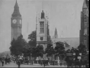
Content dump from my hiatus-ed masters degree…all very interesting, but not much context.
C++:
RayTracer
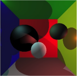
In order to get objects to cast shadows, every time an intersection is found from the primarily cast ray, a new ray (a ‘shadow ray’) is cast from the intersection point, heading towards the light source. Just like finding the initial intersection points, this ray is checked for intersection with any other objects. If the ray does have an intersection, then we know that the point is in shadow. Multiple lights can be addressed by looping over total number of lights in the scene.
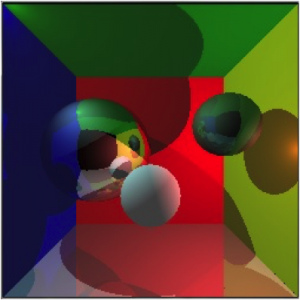
Reflections are performed by casting rays originating from the intersection point, directed along the computed reflection vector. A portion of the reflected ray’s color will be contributed to the original intersection point.
The direction calculation is:
R = -E + 2(N.E)N (N & E are normalized)
Where:
R = reflected ray
E- incidence ray
N- normal
where kr = ks (specular reflectance).
Shadow: Reflection:
Polygon Clipping
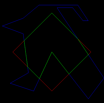
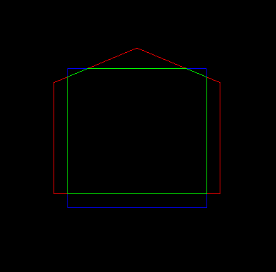
Implementation of the Sutherland-Hodgman clipping algorithm.
A test for intersection is performed between each clip window vertex in the array and each subject polygon vertex in the array and the data is stored. A temporary array is created to store the unclipped polygon as it undergoes the clipping process. Vertices of new shape are sent to the temporary array while computing, then output to the final shape for display.
Sutherland Hodgman only accepts convex clipping windows, as the algorithm relies on the turn of the clipping region to determine what is inside and outside the region. Convex shapes have constant turn. If each edge is followed counter-clockwise it will always turn left to the next edge. In other words, if a point is to the left of all clipping edges (following the edges counter-clockwise), then it is inside the clipping region. If a point is to the right of any clipping edge, then it is outside the clipping region and can be eliminated.
Scene Graphs/OpenGL
Components:
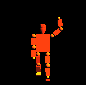
Head (obj file)
Torso (cube primitve)
Limb (cube primitive): Upper & lower arms & legs
Ball joints (sphere primitive): Shoulders, elbows, knees, hips, ankles Feet (cube primitve)
Dependency trees:
Shoulder -> Limb (UA) -> Elbow -> Limb (LA) -> Hand
Hip -> Limb (UL) -> Knee-> Limb (LL)-> Ankle -> Foot
Animations enabled:
Simple wave. Upper arm (and by extension, lower arm) raises along y axis, forearm moves along x axis from elbow in a wave.
Walking enabled by moving each limb appropriately using triggers that cease when the angle of the limb reaches a cut off point, restarting again where appropriate.
Info:
The robot components are made of minimal primitives, with transforms applying to the points/vertices of each object
Local transform:
An object’s local transformation maps LC to the parents LC (e.g. lower arm to upper arm via elbow joint). Directions e.g. up depend on what transformations have been defined by ancestors in the tree.
Implementation is carried out by push and pop matrices (recursive descent) – push being used on graph descend and pop being used on graph ascend. The concatenation of all local transform matrices is called the current transformation matrix (CTM). Each node other than root contains a piece of geometry e.g. a limb or joint. Each link is a transformation matrix. The robot can be posed by changing rotation in the joints e.g. shoulder and elbow. E.g. to draw a leg, the entire leg would be drawn within one push matrix, with the upper and lower sections being separated by another push matrix (a graph descent within a graph descent), making a dependent tree of positioned primitives.
MatLab:
Image Processing
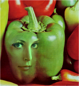
The values of specific pixels need to be altered to get a solution to this problem, in order to make image B more like image A. The pixels on the boundary of image B need to be to be equal to the pixels on image A where B resides, and then we can solve for the rest of the pixels on the interior of image B that preserve the original gradient of image B.
Poisson Image Editing starts out thinking of image A and image B as continuous functions in 2D space, and formulating/solving a partial differential equation that describes the implantation of the gradient of image B onto image A in a least squared sense. The aim is to solve for a new image that matches the background of image A better, and the border of this new image matches up with image A exactly, while the difference between adjacent points of the new image matches up with the difference of the corresponding adjacent points in image B.
To solve for the pixels in the interior of the new image, the gradient of the pixels on the interior of the new image must be equal the gradient of the pixels on the interior of image B. A simple way to define a gradient of an image at a spot is the sum of the differences between that pixel and all of its neighbours: If one of the neighbours happens to be a boundary pixel, then its value is fixed. If one of the neighbours happens to be out of bounds of the selection, then it should be excluded.
We have to compute everything simultaneously, which can be done by solving the matrix equation x = A\b. The size of both vectors x and b is the number of pixels in the target image. The vector x contains all pixels in the final image (what we are solving for). The vector b is the guiding gradient plus the sum of all non-masked neighbour pixels in the target image. The non-masked neighbour pixels define the value of the pixels at the boundary of the mask, which are blended across the mask area. The guiding gradient defines the second derivative of the final pixels in the mask area, and helps to “shape” what is blended in the mask area. The matrix A is a sparse matrix, which computes the gradient of the masked pixels in the final image. To get the final image, simply solve the equation for x. If the guiding gradient is zero, we are just solving a Laplacian equation, and the values at the mask boundary are blended smoothly across.
Region Filling
Implementation of a region filling algorithm. Smoothly interpolates inward from the pixel values on the outer boundary of the region of interest (polygon) selected. Computes the discrete Laplacian over the regions and solves the Dirichlet boundary value problem.
For every pixel outside the masked region, the equation is simply the identity: output pixel equals input pixel. For every pixel inside the masked region, the pixel value should equal the average of the pixel values of its north, east, south, and west neighbours.
Solved using sparse matrix equation x = A\b (mentioned above).

Seamless Cloning

Video Processing
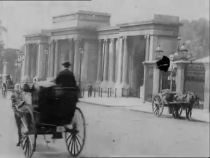
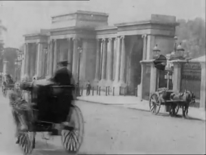
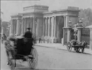
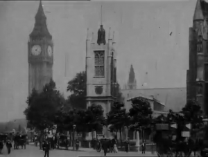
Restoring Old Film
Detection of scene cuts:
As they will simply appear as hard transitions since old films don’t display effects to switch from a scene to another, we can use imabsdiff to calculate the Absolute difference of two images (in this case, video frames). If there is a significant change, the relevant frame is considered a scenecut.
d = imabsdiff(film2,film1) subtracts each element in array film2 from the corresponding element in array film1 and returns the absolute difference in the corresponding element of the output array d.
Correction of global flicker:
As intensity flicker is an unnatural temporal fluctuation in perceived image intensity, to reduce intensity flicker, we can adjust the image mean towards a local (mean from temporally close images). This should achieve a more uniform global luminosity over time. The algorithm detects significant change of the histogram between frames, and considers these frames as global flicker. Ignoring the scene cut and very large histogram change that maybe caused by moving objects, the remaining big changes between frames can be considered as global flicker. The mean pixel values of the temporally close frames can be calculated, and the image mean adjusted by adding the difference back. Histogram equalisation was also attempted but did not achieve as satisfactory results.
Correction of blotches:
Dirt detection typically involves two generic steps, namely the identification of inconsistency of a pixel in relation to its spatio-temporal neighbourhood followed by thresholding. The first step is conventionally implemented by a suitable combination of intra/inter type of filtering. In the second step a well-established principle is that the choice of threshold will influence the balance between false alarm rate and correct detection rate.
In temporal filtering approaches, dirt is viewed as a temporal impulse (single-frame incident) and hence treated by inter-frame processing by taking into account at least three consecutive frames. In spatio-temporal filtering, pixel inconsistency is determined by the examination of both spatial and temporal neighbourhoods (at least 3 consecutive frames).
This function firstly selects pixels that differ from previous and next frames by detecting the absolute difference, and takes the results as potential blotches. This method is more suitable than creating a binary image, as there are both blotches of ‘sparkle’ and ‘dirt’, making it a suitable masking method to highlight blotches in archival film. It then detects the pixels that are caused by the motion, by finding if this pixel is similar to its right or left side neighbours from the previous and next frames. After subtracting the motion pixels, the pixels that are not detected as blotches from the previous and next two frames in the temporal neighbourhood are selected to fix the blotch pixels.
Correction of vertical artefacts:
To fix the images in the last scene without blurring them, vertical median filtering can be applied alongside unsharp masking. Median filtering is a nonlinear operation often used in image processing to reduce “salt and pepper” noise. Median filtering is more effective than convolution when the goal is to simultaneously reduce noise and preserve edges. B = medfilt2(A,[m n]) performs median filtering of the matrix A in two dimensions. Each output pixel contains the median value in the m-by-n neighborhood around the corresponding pixel in the input image. medfilt2 pads the image with zeros on the edges, so the median values for the points within [m n]/2 of the edges may appear distorted.
In this algorithm, medfilt2 was adjusted by setting one of the dimensions to have size 1, meaning that the filter is working in 1x n pixel neighbourhoods to remove vertical artifacts. To fix the artifacts without blurring the image as a result, Unsharp masking is used to save the details of edges, and added back to reduce the blurred result. The unsharp masking technique comes from a publishing industry process in which an image is sharpened by subtracting a blurred (unsharp) version of the image from itself.
B = imsharpen(A) returns an enhanced version of the grayscale or truecolor (RGB) input image A, where the image features, such as edges, have been sharpened using the unsharp masking method.
B = imsharpen(A,Name,Value,…) sharpens the image using name-value pairs to control aspects of unsharp masking.
Correction of camera shake:
This simplified algorithm uses the results of Sobel edge detection of two frames to calculate their 2D cross-correlation, using Matlab’s xcorr2 function. C = xcorr2(A,B) returns the cross-correlation of matrices A and B with no scaling. xcorr2 is the two-dimensional version of xcorr. The location of the maximal correlation in 2D can be seen as the feature position, representing the whole frame’s location.
The first frame calculates the 2D cross-correlation with itself as the reference frame. The 2D cross-correlation is then calculated between the second frame and the first frame, and so on. By comparing the result location with the reference location, whether the second frame has shaken can be detected. Afterwards the potential camera shake can be recovered by moving the second frame to the right position.
